Quick Start
This walkthrough uses the sample cell and valve entries that ship with the tool, so you can complete it without having any data of your own. It takes about ten minutes and costs one solver run against your plan.
At the end you will have a result you can compare against the numbers printed below, digit for digit. If yours match, the tool is behaving and you have read the interface correctly.
Step 1: Open the Tool
Go to prv.thermosketch.com and sign in. The workspace loads with three columns:
- Input Parameters on the left, where you describe the case
- Results Visualization in the centre, where the charts appear
- Key Results on the right, where the headline numbers appear
Underneath the charts is a Messages console. Watch it while the page
loads. It should report Databases loaded: 2 cells, 2 valves. If it reports a
failure instead, see Troubleshooting.
Step 2: Set the Pack and Ambient Conditions
In the left column, under Battery Pack Geometry and Working Conditions, set these values. Most of them are already the defaults.
| Field | Value | Unit |
|---|---|---|
| Void Volume in Pack | 30 | L |
| Max Pressure Limit | 50 | kPa |
| Ambient Pressure | 101.325 | kPa |
| Initial Temperature | 25 | °C |
| Temperature Mode | Assumed Constant |
Two of these are worth understanding before you move on.
Void Volume in Pack is the free gas volume inside the sealed enclosure, not the enclosure’s external volume. Subtract the cells, modules, cooling plates, and everything else solid. This value directly scales how fast pressure rises, so a rough guess here produces a rough answer.
Max Pressure Limit does not affect the simulation at all. It is the threshold the tool compares your result against, expressed relative to ambient, and it drives the pass or fail verdict and the assessment column in the PDF report. It comes from your enclosure structural analysis or burst test, not from the valve.
Step 3: Choose the Cell Venting Data
Under Cell Venting Data, leave Data Source on Database, then click
Browse database…. Select Demo-NCM-40Ah, from Demo Company, and close
the dialog. The selection line under the button should read
Demo-NCM-40Ah, Demo Company.
Leave Number of Venting Cells at 1.
Look at the Simulation Time (s) field in the top toolbar. It should now
read 25. The tool sets it from the length of the venting curve you selected,
which is 15 s, plus 10 s so the run continues past the end of venting and you
can watch the valve close and the pressure fall back. Once you type a value
there yourself, the tool stops adjusting it.
The built-in cell and valve entries are fabricated sample data, provided so you can learn the workflow. They are not measurements of any real product and must not be used for design decisions. See Input Data Sources.
Step 4: Choose the Valve
Under Pressure Relief Valve Characteristic, leave Data Source on
Database, click Browse database…, and select S001, from Demo
Company. It is a spring valve with a 5 kPa opening pressure. The dialog also
previews its two flow curves, one for the closed valve and one for the open
valve.
Leave Number of Valves at 1.
Step 5: Run
Click Run in the toolbar. The button shows Solving… while the request is
in flight, and the Messages console reports the solve when it returns.
Step 6: Check Your Numbers
The Key Results column on the right should now read:
| Metric | Value |
|---|---|
| Verdict | Pressure Within Limit |
| Absolute Peak Pressure | 108.764 kPa |
| Relative Peak Pressure | 7.439 kPa |
| Valve Opened | Yes |
| First Open Time | 1.173 s |
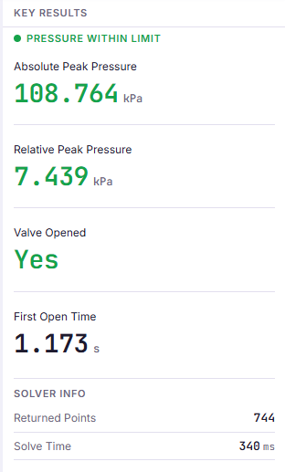
If your numbers match, you have set the case up correctly.
Read them like this. The pack peaked at 108.764 kPa absolute, which is 7.439 kPa above the 101.325 kPa ambient you specified. Your enclosure limit was 50 kPa relative, so the case passes with a wide margin. The valve opened 1.173 s into the event, which is when pressure first crossed the valve’s 5 kPa setpoint.
Note that the verdict compares the relative peak against your limit, not the absolute one. Enclosure pressure ratings are almost always quoted as a differential across the wall, which is what the relative number is.
Below the metrics, Solver Info shows how many points came back and how long the solve took. Those vary slightly between runs and carry no engineering meaning.
Step 7: Look at the Curves
The centre column has three chart layouts:
- Single Chart shows one quantity at a time, chosen from the dropdown beside the tabs
- Four Grid shows pressure, temperature, gas moles, and valve flow at once
- Vertical Stack shows the same four stacked on a shared time axis
Open Single Chart and select Pressure. You should see pressure climb from ambient, turn over shortly after the valve opens, and fall back. The flat reference line is the ambient pressure you entered.
Then open Four Grid. The bottom right panel carries two series: valve flow rate, and valve status as a 0 or 1 step. Line up the moment the status steps to 1 against the moment the pressure curve turns over. That is the whole point of the tool in one picture.
Step 8: Export, or Save the Setup
Two different things, often confused:
- Export produces results.
Export Data (CSV)gives the full resolution time series, andDownload Report (PDF)gives a formatted report with the input summary, the input curves, the result charts, and the verdict. Each export counts against its own quota. - Save / Load produces a setup.
Save Configurationdownloads a.jsonfile containing every input, including any curves you uploaded, so you can reopen the same case later. It costs nothing and never leaves your machine.
Results are not stored anywhere. If you close the tab without exporting or saving, they are gone, and the browser will warn you once before you do.
What Next
- Change Number of Venting Cells to
5and run again. The relative peak rises to 27.726 kPa, still inside the 50 kPa limit but no longer comfortable. That is the sensitivity the tool exists to show you. - Choosing a Valve turns that into a repeatable selection procedure.
- Mathematical Model explains what the solver actually integrates, so you can defend the number.